CIG-LLNL Computational Seismology Workshop

Table of Contents

1. Overview
2. Introduction
3. Part I: Setting up SPECFEM3D_GLOBE
4. Part II: Continental-scale Simulations
5. Part III: Visualization
   1. Visualize Seismograms
   2. Visualize Model Mesh
   3. Visualize Surface Movie
6. Part IV: Adjoint Simulations (Bonus)
7. Further Work
8. Resources

Part III: Visualization

In this third part of the tutorial, we will look at methods for visualizing the output simulation data. We will look at the following categories:

• Visualize Seismograms
• Visualize Model Mesh
• Visualize Surface Movie

Visualize Seismograms

The output seismograms can be found in the OUTPUT_FILES/ folder. In order to visualize the seismograms, we will use the seisplot.py script that is located in the root folder.

This script takes the names of the seismograms we want to visualize as command line input, and uses ObsPy under the hood to generate the plots. The usage is as follows:

      python3 seisplot.py [seismogram_file_names]

Since ObsPy is not available on Quartz by default, we must run it through a virtual environment. We do this by running the following command:

      alias python3 /usr/apps/specfem/python/bin/python3

Now, if we want to visualize the seismograms IU.ANMO.BXZ.sem.sac, II.PFO.BXZ.sem.sac, and IU.TUC.BXZ.sem.sac, we would type

      python3 seisplot.py ./OUTPUT_FILES/IU.ANMO.BXZ.sem.sac ./OUTPUT_FILES/II.PFO.BXZ.sem.sac ./OUTPUT_FILES/IU.TUC.BXZ.sem.sac

Which will give us the following plot:

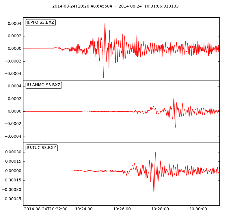
In this section, we have looked at how to plot the seismograms generated by SPECFEM3D_GLOBE.

In the next section, we will look at how to visualize the model mesh with different components (e.g. vp, vs).

Previous section – Next section